2. A Gaussian XOR problem

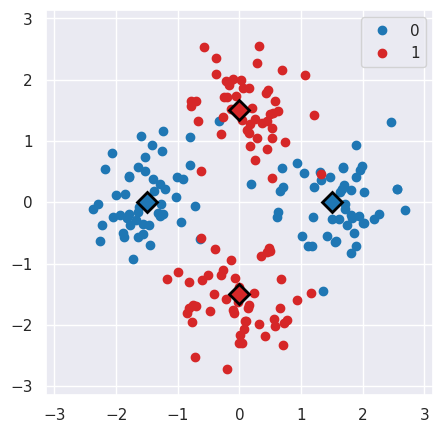
Our second example is the XOR problem. We place four points over the cartesian axes so to create a centered square; the two points on x-axis are labeled as 1, while those on y-axis as 0.

2.1. Dataset generation

We use numpy to generate a dataset of 200 points by sampling 50 points from 4 gaussian distibutions centered at the said points. The label of each sample is given by the center of its distribution.

import numpy as np

n_pc = 50 # Number of points per cluster

# Create a matrix of vertices of the centered square
X = np.asarray(n_pc * [[1.5, 0.]] +
               n_pc * [[-1.5, 0.]] +
               n_pc * [[0., -1.5]] +
               n_pc * [[0., 1.5]]
)
# Add gaussian noise
X += .5 * np.random.randn(*X.shape)

# Create target vecor
y = np.concatenate((np.zeros(2*n_pc), np.ones(2*n_pc)))

This generates the following dataset, where the circles represent the samples and the squares the distribution centers.

2.2. Circuit definition

Now, we define the circuit structure using the make_circuit function.

def make_circuit(bdr, x, params):
    """Generate the circuit corresponding to input `x` and `params`.

    Parameters
    ----------
    bdr : circuitBuilder
        A circuit builder.
    x : vector-like
        Input sample
    params : vector-like
        Parameter vector.

    Returns
    -------
    circuitBuilder
        Instructed builder
    """

    bdr.allin(x[[0,1]])

    bdr.cz(0, 1).allin(params[[0,1]])

    bdr.cz(0, 1).allin(params[[2,3]])

    return bdr

2.3. Model training

Finally, we can create and train the classifier. We instantiate the circuitML subclass that we prefer, in this case the one using the fast manyq simualtor, specifying the number of qubits and of parameters.

from polyadicqml.manyq import mqCircuitML

nbqbits = 2
nbparams = 6

qc = mqCircuitML(make_circuit=make_circuit,
                nbqbits=nbqbits, nbparams=nbparams)

Then, we create and train the quantum classifer, specifying on which bitstrings we want to read the predicted classes.

from polyadicqml import Classifier

bitstr = ['00', '01']

model = Classifier(qc, bitstr)
model.fit(X, y)

2.4. Predict on new data

We can use a model to predict on some new datapoints X_test that it never saw before. To obtain the bitstring probabilities, we can just call the model:

pred_prob = model.predict_proba(X_test)

Then, we can retrieve the label of each point as the argmax of the corresponding probabilities. Otherwise, we can combine the two operations by using the shorthand:

y_pred = model(X_test)

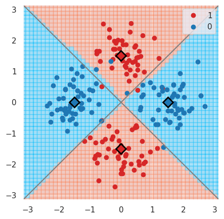
For instance, going back to our XOR problem, we can predict the label of each point on a grid that covers , to assess the model accuracy. Using some list comprehension, it would look like this:

t = np.linspace(-np.pi,np.pi, num = 50)
X_test = np.array([[t1, t2] for t1 in t for t2 in t])

y_pred = model(X_test)

We can now plot the predictions and see that the model is very close to the bayesian prediction (whose decision boundaries are shown as grey lines), which is the best possible.

2.5. Source code

The example script, producing the plots, can be found in the GitHub example page as example-XOR.py.