1. Defining a quantum circuit
The first step in running a Quantum Machine Learning algorithm consists in defining a parametric quantum circuit. A quantum circuit is a sequence of instructions, or gates, that we apply to one or more qubits, the computational units of a quantum computer. A circuit being parametric means that the gates depend on some parameters, which in our case will be real valued angles.
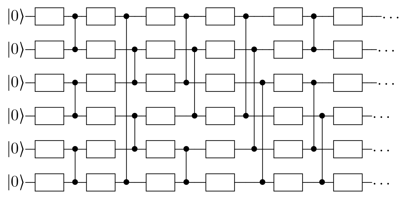
Example of a quantum circuit.
The figure gives a graphical representation of a quantum circuit.
Each line represents a qubit, to which gates are applied from the left to right.
We use rectangles to identify single-qubit gates and vertical lines,
terminating with a specific marker, to represent entangling gates,
which affect two qubits.
The leftmost symbol of each line gives the initial state of the
corresponding qubit, which we always assume to be  .
.
1.1. The circuitBuilder class
Since different quantum computer providers use different functions to implement the same operations, we resort to a circuit builder, which abstracts away the provider’s syntax.
The circuitBuilder class defines some high level methods to address
qubit operations:
input(idx,theta): Add input gate to the qubit corresponding to indexidx. This consists of a qubit rotation of .
Both
.
Both idxandthetacan be iterables; in this case, for each element oftheta, a single input gate is added to the corresponding index inidx.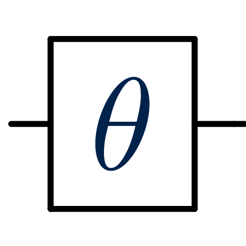
Input gate representation.
allin(theta): This operation takes a list of angles and, for each element, add an input gate to the corresponding qubit. It has the same effect asinput(range(nbqbits), theta).cz(a,b): Add CZ gate between qubitsaandb. This is a symmetric entangling gate.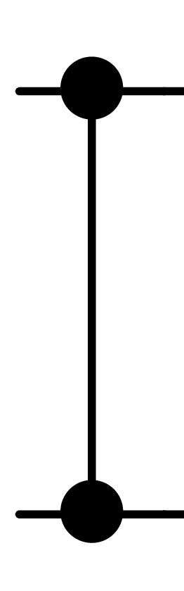
CZ gate representation.
measure_all(): Add measurement to all qubits.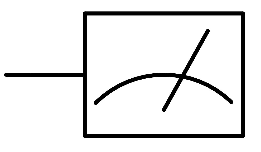
Measurement gate representation.
circuit(): This method returns the circuit completed with the provided instructions. The specific return type varies across the builder implementations, but, as we will see when discussing themake_circuitfunction and thecircuitMLclass, we never manipulate circuits directly.
1.1.1. Example
We can now build our first quantum circuit.
As circuitBuilder is an abstract class, we use for this example the
Qiskit implementation, but note that any builder would produce the same
circuit.
The Qiskit implementation is presented in depth in The Qiskit/IBMQ interface.
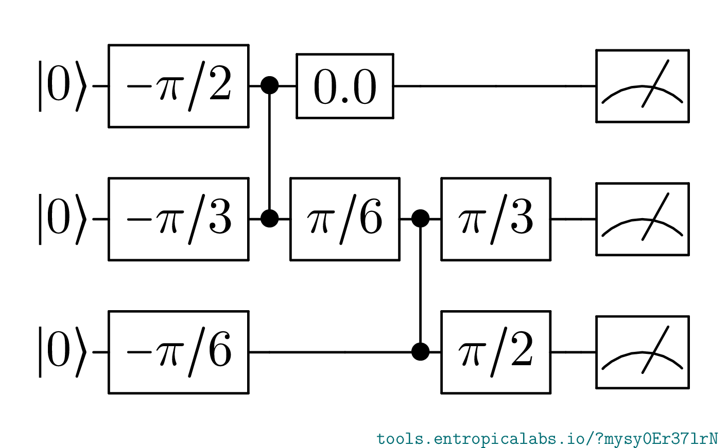
We use a vector  of size seven to define the three-qubits
circuit in figure.
of size seven to define the three-qubits
circuit in figure.
from polyadicqml.qiskit import qkBuilder
import numpy as np

# We create the vector [-pi/2, -pi/3, -pi/6, 0, pi/6, pi/3, pi/2]
theta = np.linspace(-np.pi/2, np.pi/2, 7)

# We instantiate the builder

bdr = qkBuilder(3)  # 3 is the number of qubits

# We start by inputting the first three elements of theta

bdr.allin(theta[:3])

# Then we entangle the first two qubits

bdr.cz(0,1)

# Then input el. 3 and 4 from theta in qubits 0 and 1

bdr.input([0,1], theta[[3,4]])

# Then again entanglement and input
# Note that we can concatenate instructions

bdr.cz(1,2).input([1,2], theta[[5,6]])

# Finally, we measure.
bdr.measure_all()
Now that the builder is complete, we can retrieve the built circuit
with bdr.circuit().
Furthermore, since we are using the Qiskit implementation, the return
type is a qiskit.circuit.QuantumCircuit.
We can print it and verify that it corresponds indeed to our desired
circuit:
>>> print(bdr.circuit())
        ┌──────────┐┌───────────┐┌──────────┐   ┌──────────┐ ┌───────┐  ┌──────────┐                                        ░ ┌─┐
  qr_0: ┤ RX(pi/2) ├┤ RZ(-pi/2) ├┤ RX(pi/2) ├─■─┤ RX(pi/2) ├─┤ RZ(0) ├──┤ RX(pi/2) ├────────────────────────────────────────░─┤M├──────
        ├──────────┤├───────────┤├──────────┤ │ ├──────────┤┌┴───────┴─┐├──────────┤   ┌──────────┐┌──────────┐┌──────────┐ ░ └╥┘┌─┐
  qr_1: ┤ RX(pi/2) ├┤ RZ(-pi/3) ├┤ RX(pi/2) ├─■─┤ RX(pi/2) ├┤ RZ(pi/6) ├┤ RX(pi/2) ├─■─┤ RX(pi/2) ├┤ RZ(pi/3) ├┤ RX(pi/2) ├─░──╫─┤M├───
        ├──────────┤├───────────┤├──────────┤   └──────────┘└──────────┘└──────────┘ │ ├──────────┤├──────────┤├──────────┤ ░  ║ └╥┘┌─┐
  qr_2: ┤ RX(pi/2) ├┤ RZ(-pi/6) ├┤ RX(pi/2) ├────────────────────────────────────────■─┤ RX(pi/2) ├┤ RZ(pi/2) ├┤ RX(pi/2) ├─░──╫──╫─┤M├
        └──────────┘└───────────┘└──────────┘                                          └──────────┘└──────────┘└──────────┘ ░  ║  ║ └╥┘
meas_0: ═══════════════════════════════════════════════════════════════════════════════════════════════════════════════════════╩══╬══╬═
                                                                                                                                  ║  ║
meas_1: ══════════════════════════════════════════════════════════════════════════════════════════════════════════════════════════╩══╬═
                                                                                                                                     ║
meas_2: ═════════════════════════════════════════════════════════════════════════════════════════════════════════════════════════════╩═
1.2. The make_circuit function
We just learned how to use a circuitBuilder to build a circuit.
Nonetheless, in machine learning, we are interested in running the same
circuit architecture with many different inputs and many different
parameters.
It is obvious that writing a new builder for each change in numerical
values would be a tedious and useless task.
Although, if we recall our previous circuit example, we notice how with
can easily substitute the vector theta with a variable, as in the
builder methods we only refer to it through its indices.
This idea motivates the introduction of the make_circuit function,
whose documentation we report here:
As we see, this function makes an explicit distinction between input and
model parameters, respectively x and params.
Furthermore, the function signature has to respect the precised one,
by taking a builder, alongside the input and parameters vectors, and
returning an instructed builder.
Therefore, the implementation of a make_circuit function proceed as
follows, where we see highlighted the important parts.
def make_circuit(bdr, x, params):

    ... # Series of instruction for the builder, e.g:
    bdr.input([0,1], x[[0,1]]).cz(0,1)
    bdr.input([0,1], params[[0,1]])
    ...

    # Return the instructed builder
    return bdr
This function is the only place in which we talk to quantum circuits – even
if indirectly.
In fact, we give this function to a circuitML, which will handle the
backend, without having to worry about the shape of the internal
representation.
Note
We usually avoid adding measure gates – measure_all() – in
the make_circuit function, as we do not know in advance if we are
working with the actual circuit output (i.e. the measurement) or
with the simulated quantum state.
In fact, measurement would collapse the quantum state, so its amplitudes, which we are interested in, would not be the bitstring probabilities anymore, but a mere sample.
Again, this is handled by the circuitML class, explained next.
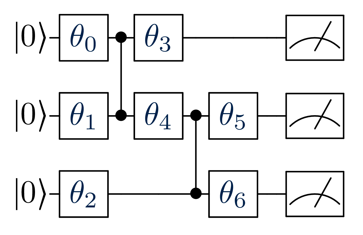
1.2.1. Example 1
As first example, we just translate the circuitBuilder example, so that
 will now be any possible parameter vector
params, as shown in the figure.
def make_circuit(bdr, x, params):

    # We pipeline some of the previous instructions
    # Note that `theta` has become `params`
    bdr.allin(params[:3])
    bdr.cz(0,1).input([0,1], params[[3,4]])
    bdr.cz(1,2).input([1,2], params[[5,6]])
Note that this circuit is independent from the input vector x, as it
is not used, but it is still required in the function signature.
We can obtain the same circuit as in previous example by calling
make_circuit(qkBuilder(3), [], theta).measure_all().circuit()
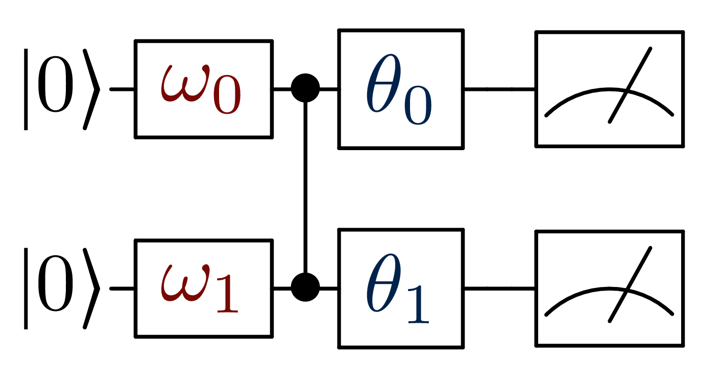
1.2.2. Example 2
For the second example, we define a circuit on two qubits, for
four-dimensional data.
The circuit has eight parameters and its structure is repetitive, which we
can leverage with the functional nature of make_circuit and the builder.
The figure represents the desired circuit, where  represents the input vector
 x; the red rectangles highlight the
repeated block.

# We define a block function, as the structure is repetitive
def block(bdr, x, p):
    bdr.allin(x[[0,1]])
    bdr.cz(0,1).allin(p[[0,1]])

    bdr.cz(0,1).allin(x[[2,3]])
    bdr.cz(0,1).allin(p[[2,3]])

def make_circuit(bdr, x, params):
    # The fist block uses all `x`, but
    # only the first 4 elements of `params`
    block(bdr, x, params[:4])

    # Add one entanglement not to have two adjacent input
    bdr.cz(0,1)

    # The block repeats with the other parameters
    block(bdr, x, params[4:])

    return bdr
1.3. The circuitML class
The circuitML class provides the interface to run multiple parametric
circuits with different inputs and model parameters.
We report its documentation:
This is an abstract class, so we cannot directly instaciate it, but it
fixes the interface.
As we see, the constructor requires four arguments: make_circuit,
nbqbits, nbparams, and cbuilder.
The first argument, make_circuit, corresponds to the function from
previous section, which circuitML will access as if it was an internal
method; thus the documentation provides the signature.
The latter, cbuilder, is the class (and not an instance) of the
circuit builder to be used; as each child class knows its own backend
implementation, this argument is provided by default.
The main method of this class is run, which takes as input a design
matrix X and a parameter vector params and runs each
corresponding circuit.
People in quantum computing know that, given a circuit, we transform a
quantum state into another.
Nonetheless, the final quantum state is not accessible in an actual
quantum computer; we measure each qubit, which reads either 0 or
1.
The output of each mesurement is thus a binary sequence of length
nbqbits, a bitstring, which follows a probability distribution
given by the quantum state.
For each run, the quantum computer executes the circuit many times,
in what we call shots.
The run output is thus a sequence of nbshots bitstrings, which
gives a statistic of the underlying distribution.
Therefore, the output of a run call will be an array.
Each row corresponds to the run of the circuit given by the input sample.
Each row entry – i.e. each column – gives the number of times the
corresponding bitstring appeared in the shots, i.e. its counts.
That said, with enough computing power, it is possible to simulate
quantum computers with a small number of qubits and retrieve the actual
bitstring distribution.
In that case, we can exactly compute the bitstring distribution.
When possible, this corresponds to calling run with nbshots=None,
which is also the default value.
1.3.1. Example
We define a simple circuit, then, we run it for two different input points. The 2-qubit circuit in figure takes a bidimensional input and two parameters, which will be fixed.
We use the manyq implementation, which relies on a simulator and is
explained in detail in The manyq simulator.
We need to define the make_circuit and then we can instantiate the
circuitML.
# `make_circuit` can have any name
def simple_circuit(bdr, x, params):
    return bdr.allin(x).cz(0,1).allin(params)

# We instantiate the circuitML
from polyadicqml.manyq import mqCircuitML

circuit = mqCircuitML(simple_circuit, nbqbits=2, nbparams=2)
Now that we have a circuit, we can run it. As we are using a simulator, we have acces to the probability distribution, from which we get counts realizations.
# We create an input matrix and a param.s vector
import numpy as np

X = np.array([[-np.pi/4, np.pi/4],
            [np.pi/4, -np.pi/4]])
params = np.array([np.pi/2, -np.pi/2])

# We retrieve the probabilities and a realization of the counts
probs = circuit.run(X, params)
counts = circuit.run(X, params, nbshots=100)
We show in the figures the probability distribution for the two samples
we considered and a count realization over 100 samples that we obtain by specifying nbshots=100.

Bitstring probabilities

Bitstring counts over 100 shots