2. The polyadicQML `Classifier`¶

In the previous tutorial we learned how to define a runnable parametric quantum circuit using circuitML. Here, we will integrate a parametric circuit in a classification model, train its parameters and predict the classes of new samples. All of this is easily done using a Classifier.

For people familiar with the popular python package scikit-learn, the syntax will be very familar, as we rely on two methods: fit and predict. To explain each step of this tutorial (Creating a Classifier, Training the parameters, Predicting on new points), we rely on a simple example: the binary classification of points generated from two gaussians on the plane, which we show in figure.

Two clusters of binary points in two dimensions.¶

2.1. Creating a Classifier¶

To define a classifier, we need two ingredients: a circuitML and a list of bitstrings. The former is the circuit we intend to use in our quantum classifier. The list of bistrings specifies on which bitstring we want to read the classes.

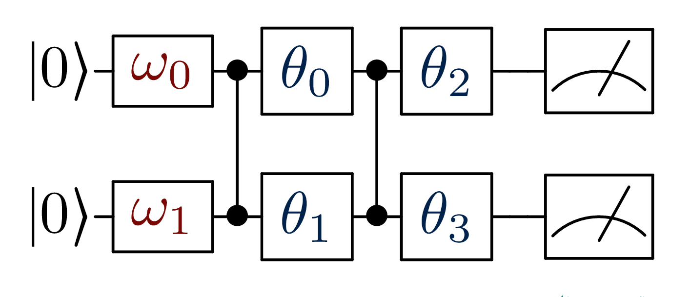
Parametric quantum circuit on two qubits

Imagine we want to use the simple circuit represented in figure, to classify the binary dataset. Again, $\omega$ encodes for the input vector x and $\theta$ represents the models parameters.

The first step requires to create a circuitML, as seen in previous tutorial. We use the manyq implementation.

# We define the circuit structure
def simple_circuit(bdr, x, params):
    bdr.allin(x).cz(0,1).allin(params[:2])
    bdr.cz(0,1).allin(params[2:4])
    return bdr

# We instantiate the circuit
from polyadicqml.manyq import mqCircuitML

nbqbits = 2
nbparams = 4

qc = mqCircuitML(make_circuit=simple_circuit,
                 nbqbits=nbqbits, nbparams=nbparams)

Now, we have to choose on which bitstrings to read the classes. Since we are using two qubits, the circuit can generate four different outputs, as the number of possible bitstrings is $2^{\text{nbqbits}}$ and $2^2=4$ . The bitstring choice is arbitrary and different readouts creates different decision boundaries. Nonetheless, we can guide our choice using heuristic arguments. For instance, choosing to assign 00 and 01 to class 0 and 1 respectively, would mean that our model output should always keep the first qubit ‘inactive’, while using the second one to discriminate the classes. A more thoughtful choice, in this case, could be to choose a pair of reversed bitstrings, such as 01,10 or 00,11, so that a change in the class can be interpreted as a flip of state on the output qubit.

We choose to go with 00 and 11 and we instantiate the classifier. By default, the classifier uses the exact quantum-state probabilities, to use shots-based probabilites, one should specify the nbshots keyword argument in the constructor.

from polyadicqml import Classifier

bitstr = ['00', '11']

model = Classifier(qc, bitstr)

Note

The number of shots and the circuitML implementation can be changed at any time through the nbshots attribute and the set_circuit methods. This is very useful to train models on simulators and then testing them on real hardware.

2.2. Training the parameters¶

Parameter training is straightforward and only requires a call to the fit method, by providing the design matrix X and the corresponding labels y.

model.fit(X, y)

Parameters are optimized to minimize the negative loglikelihood.

On top of that, fit accepts many different optional parameters. The first one, which can be positional, is the batch_size, which tells how many samples, picked at random, should be used at each iteration to compute the loss.

The most important keyword argument is method, a string that specifies the numerical optimization method to be used. For now, polyadicQML relies on the SciPy optimization module and therefore, supports all methods provided by scipy.optimize.minimize; nevertheless, we mainly rely on BFGS and COBYLA, the former being the default method.

BFGS is a gradient based method, which we compute using finite differences. With this approach, there is no reliable way to approximate the gradient with a limited number of shots. Therefore, to train a quantum model which do not use the bitstring probabilities from the quantum state, but estimates them through shots, we must resort to a gradient-free method, such as COBYLA.

For instance, we can choose to use shots by specifying it in the Classifier constructor. In this case, we should be aware of the optimization method.

model = Classifier(qc, bitstr, nbshots=300)
model.fit(X, y, method='COBYLA')

Loss progress during model training.¶

2.3. Predicting on new points¶

The model being trained, we can use it to predict the label of any new point from the same space as the original dataset. Supposing we have a matrix X_test, we can predict its labels by calling the predict method.

labels_test = model.predict(X_test)

An equivalent, but shorter, version consists of directly calling the model.

labels_test = model(X_test)

For instance, the figure shows the predicted label for each point in $[-\pi,\pi] \times [-\pi,\pi]$ .

Predicted label for each point in $[-\pi,\pi] \times [-\pi,\pi]$ ; grey line is the bayesian decision boundary.¶

We can also predict the probabilities of the bitstring associated to each class, using predict_proba.

probas_test = model.predict_proba(X_test)

If we want to compute the circuit output, full and raw, we can use the run_circuit method. It returns the counts – or probabilities – of all bitstrings. For example, we can compute a realization with 300 shots over the training set X, to se how the model fits the data.

# Changing nbshots from None changes from exact probabilities
# to shots-based estimation
model.nbshots = 300

# We get the counts from each bitstring
full_output = model.run_circuit(X)

Bitstring counts over 300 shots for the training set, from run_circuit.¶

We plot the counts for each point of the two classes, along with their box plot.

2. The polyadicQML Classifier¶

2.1. Creating a Classifier¶

2.2. Training the parameters¶

2.3. Predicting on new points¶

2. The polyadicQML `Classifier`¶